All content here is for research and educational purposes only, not financial advice.

Monetising Volatility Risk Premium for AAPL
Volatility Risk Premium (VRP) refers to the difference between the Implied Volatility (IV), that is forward-looking and derived from option prices, and the Realised Volatility (RV) that is the actual variance that is realised over time (Feunou, 2017). A common observation is that IV is usually larger than RV, which indicates opportunity to capitalise on the premium from the difference between IV and RV, which is the VRP.
\[\mathrm{VRP} \equiv \mathrm{IV} - \mathrm{RV}\]For this series of VRP-type strategy research, we start with studying a large-cap stock, Apple (Ticker: AAPL), with relevant datasets retrieved through the Wharton Research Data Services (WRDS). We study its VRP to derive a basic signal for a corresponding Put Option strategy that is viable for a retail trader. In a subsequent series, we then study the risk management measures as well as other possible strategies.
Research Parameters
For this study, we anchor our parameters using AAPL put options of ~10DTE (10 Calendar Days / 7 Trading Days), with a hard minimum of 8DTE and maximum of 12DTE, with the following reasons:
-
Liquidity
10DTE options present sufficient liquidity for a more optimal bid-ask spread as well as sufficient order-book depth. This ensures fill quality, reduces slippage, and is realistically testable and executable. -
Dampened Gamma Risks
10DTE options exhibit materially lower gamma exposure than short-dated contracts, reducing gamma-driven PnL variability, and allowing theta decay to remain a more meaningful and systematic contributor to the overall strategy returns.
The date range for the data that we study is between 1 Jun 2022 and 31 Dec 2024, or what I categorise as Post-COVID-19 Regime.
We also make sure to avoid any lookahead biases so that the outcomes are implementable in reality.
Derivation of IV, RV and VRP
We use OptionMetric’s Ivy DB US Option Volatility Surface dataset to derive the annualised IV from 10DTE near-ATM AAPL put options (Δ ≈ −0.50), and corresponding AAPL spot prices from Centre for Research in Security Prices (CRSP) datasets to derive the annualised RV over 7 trading days rolling windows. Thereafter, the VRP is derived.
7-Day Annualised RV
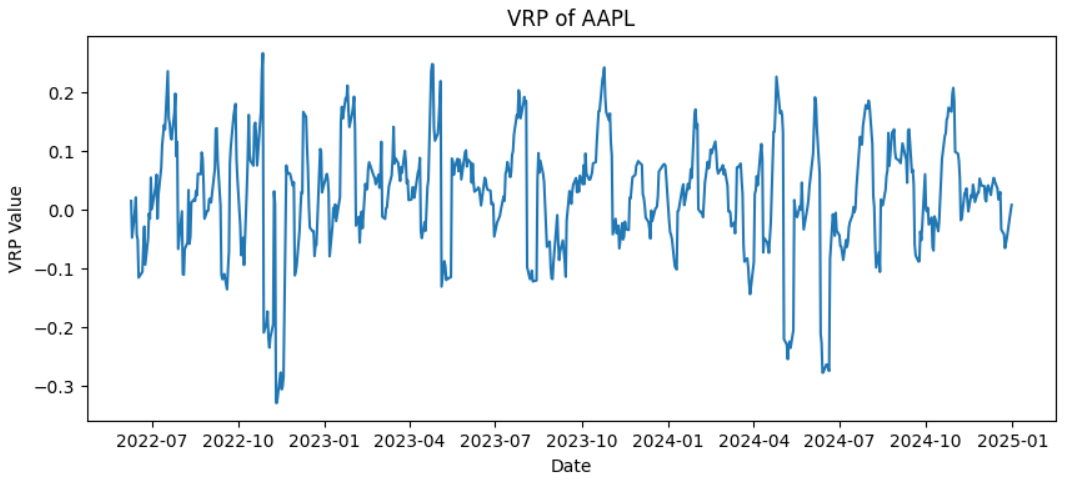
\[\begin{aligned} r_t &= \frac{P_t - P_{t-1}}{P_{t-1} } \qquad\qquad \mathrm{RV}_t^{(7)} &= \sqrt{\frac{252}{7} \sum_{i=0}^{6} r_{t-i}^2} \end{aligned}\]Figure 1: Volatility Risk Premium for AAPL
Analysis of VRP
The VRP of AAPL was plotted over time, with plausible stationarity observed.
Figure 2: VRP Over Time
We move on to examine the temporal dependence of VRP by computing the sample autocorrelation function (ACF) across multiple lags.
\[\rho(k) \;=\; \frac{\mathbb{E}\!\left[(X_t - \mu)(X_{t-k} - \mu)\right]} {\mathbb{E}\!\left[(X_t - \mu)^2\right]}\]Table 1: AR(1) estimation results for the VRP series.
| Lag | 0 | 1 | 2 | 3 | 4 | 5 | 6 | 7 | 8 | 9 |
|---|---|---|---|---|---|---|---|---|---|---|
| ACF | 1.0000 | 0.8327 | 0.6529 | 0.4904 | 0.3290 | 0.1834 | 0.0336 | -0.0996 | -0.0797 | -0.0485 |
Augmented Dickey–Fuller Test
- Test statistic: −5.98
- p-value: 1.84 × 10⁻⁷
- 1% critical value: −3.44
Given the autocorrelation values, it can be seen that the VRP has strong short-term persistence, and gradually decays to 0 within 10 calendar days and is therefore mean-reverting. This can been seen by the high first-order autocorrelation function parameter ≈ 0.8327 and an autocorrelation close to 0 at lag 7 (AR(7) ≈ -0.0996, consistent with a stationary, mean-reverting process.
We further assess stationarity using the Augmented Dickey-Fuller (ADF) test, which tests the null hypothesis of a unit root against the alternative of stationarity. Since the ADF statistic value is less than the critical values, and has a p-value of 0.000001, we can reject the null hypothesis of a unit root, and conclude that there is strong statistical evidence that the VRP series is stationary over the sample period.
These provide motivation for modelling VRP as a time-series, which will provide insights into effective timing and sizing of volatility trades, allowing the trader to systematically monetise mispricing while managing exposure to risk.
Modelling VRP as a Time-series
We now model VRP using AR(1) given the pronounced first-order autocorrelation, and confirm if the model is statistically useable, before determining the long-run mean and half-life to understand if monetising VRP will reap positive PnL, as well as the decay rate of volatility spikes. The total number of observations is 644 for this model.
\[\mathrm{VRP}_t = \alpha + \phi \, \mathrm{VRP}_{t-1} + \varepsilon_t, \qquad \varepsilon_t \sim \mathcal{N}(0, \sigma^2)\]| Parameter | Estimate | Std. Error | z-stat | p-value | 95% CI |
|---|---|---|---|---|---|
| Intercept ($\alpha$) | 0.0042 | 0.0020 | 1.89 | 0.059 | [−0.000, 0.009] |
| AR(1) ($\phi$) | 0.8327 | 0.0220 | 38.14 | < 0.001 | [0.790, 0.876] |
Long-run mean (unconditional mean)
The long-run (unconditional) mean for an AR(1) process is:
\[\mu \equiv \mathbb{E}[X_t] = \frac{\alpha}{1-\phi}.\]Half-life of mean reversion
Define the half-life (h) as the number of periods it takes for a deviation from the long-run mean to decay by 50%.
For an AR(1), deviations decay geometrically:
Setting the deviation decay factor equal to one-half:
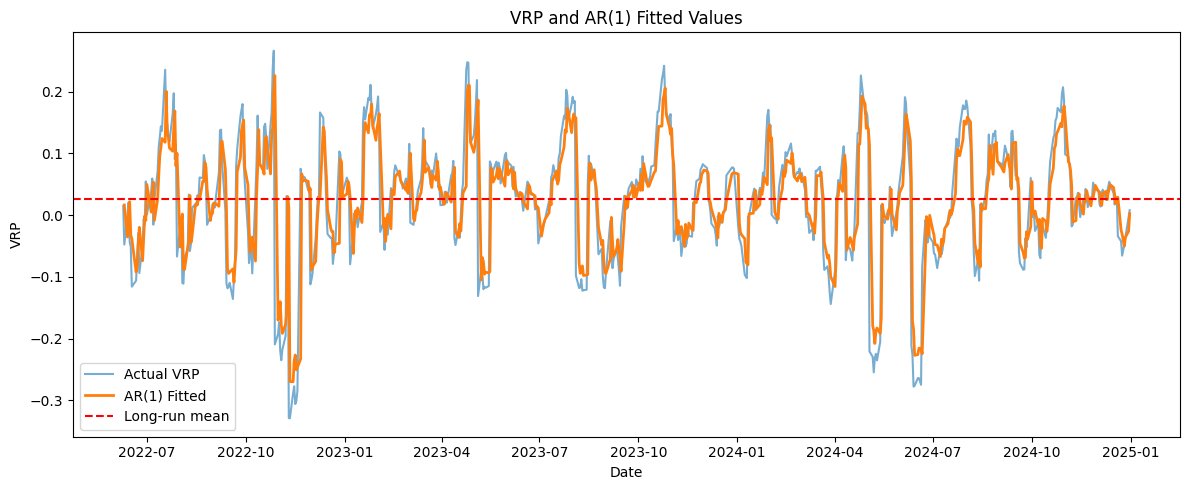
\[|\phi|^h = \frac{1}{2}\] \[h = \frac{\ln(1/2)}{\ln|\phi|}.\]Based on the results, we have an AR(1) modelled VRP that is mean-reverting with an implied half-life of approximately 4 days. The statistically significant intercept also allows us to derive the long run mean of the VRP to be at 0.0254, consistent with structural overpricing of short-dated equity options. This provides motivation for short-horizon volatility selling strategies to monetise the decay of mispricing.
Of note, we should not expect the model to provide forecasts of VRP, as the AR(1) process only factors in effects of the previous day’s VRP, and at horizons beyond one week, we should expect reversion to the long run mean of 0.0254. The knowledge of half-life will guiding the strategy’s holding period.
Figure 3: Modelled VRP against Actual VRP
Monetising VRP Using Naked Puts
We first study a pure approach to monetising VRP through the writing of put options at around 10DTE without considering risk management controls.
We obtain the dataset from WRDS OptionSuite to get the option contracts in the same date range. We also filtered for the maturity to be less than or equals to 12 days to align closely to our 10DTE analysis. Here, we select the contracts with deltas closest to -0.50 each day, as well as DTE closest to 10DTE, accepting 8DTE and 12DTE as the minimum and maximum respectively.
We start with a simple rule where a trade (put option sold) is executed on t+1 when VRP > 0 at close on time t. We align the ideal holding period with the derived half-life of 4 days minimally before the trade is exited. If t+4 days is a non-business day, or if there is no liquidity based on WRDS dataset, then the next business day or the next available trade day is when the put option is bought back. To note, we assume only one contract is traded each time.
Results of Simulated PnL
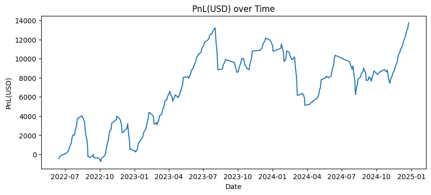
Figure 4: Cumulative PnL over Time
| Metric | Value |
|---|---|
| Sample period | 1 Jun 2022 – 31 Dec 2024 |
| Total number of trades | 341 |
| Total PnL (USD) | 13,754.50 |
| Maximum drawdown (USD) | 8,071.50 |
| Calmar ratio | 1.7041 |
Over the period of 1 Jun 2022 to 31 Dec 2024, a total of 341 trades (An entry + exit pair is considered 1 trade) were executed, with a total PnL of USD13,754.50 generated. PnL is attributed to the trade entry date to reflect the timing of risk deployment rather than exit realization.
Despite positive aggregate performance, the strategy exhibits a substantial peak-to-trough maximum drawdown of USD 8,071.50, indicating significant path-dependent risk. The resulting Calmar ratio of 1.70 suggests that while returns are positive, they are achieved with considerable drawdown exposure, highlighting a relatively aggressive risk profile that warrants further risk-management refinement.
Assuming a starting capital of USD50,000, suitable for an entry/intermediate retail trader, as well as an annualised risk-free rate of 3%, the calculated Sharpe ratio (capital-based) and Kelly Criterion are as follows:
| Metric | Value |
|---|---|
| Sharpe ratio | 0.0622 |
| Kelly fraction | 0.1828 |
The Sharpe ratio indicates weak risk-adjusted performance, while the Kelly fraction provides a theoretical upper bound on capital allocation under the assumption of stable return distributions.
Testing for Regime-resilience
A truly useful strategy is one that stands the test of time and events. So we put the strategy to test by backtesting through a different date range to understand if the strategy and signal is regime-resilient. The backtested date range is 1 Jan 2018 to 31 May 2022, which includes Pre-COVID-19 and stretches through the peak of the COVID-19 pandemic.
Figure 5: Cumulative PnL over 1 Jan 2018 to 31 May 2022
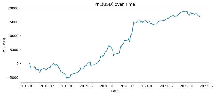
A total number of 256 trades were executed over 1 Jan 2018 to 31 May 2022 (4.5 years), with a total PnL of USD17,107.50 generated. The max drawdown is USD5,635.50 and corresponding Calmar ratio is 3.0357. This also indicates the likelihood that the strategy can still reap profits amidst elevated uncertainty.
Conclusion
Monetising VRP is a widely recognised baseline approach to generating PnL. Conceptually, it is often likened to insurance sellers who earn premiums by providing their clients protection against perceived risks that, on average, exceed their realised likelihood or magnitude.
This approach to monetise VRP through systematic put writing (capped at at most one trade per day) is readily implementable by retail traders. However, at this stage of the analysis, the primary limitation lies in the absence of explicit risk management mechanisms. In particular, short naked put positions expose the trader to adverse delta and gamma dynamics during sharp market moves. While the strategy benefits from premium collection under normal conditions, downside losses can be substantial in extreme scenarios. There is also opportunity to finesse the signal better, going beyond the simply defined VRP > 0 signal.
I will explain the risks of this strategy, and consider appropriate risk management measures in a subsequent series.
Citations
Feunou, B., Lopez Aliouchkin, R., Tédongap, R., & Xi, L. (2017). Variance premium, downside risk and expected stock returns (No. 2017-58). Bank of Canada.
PS: GenAI was used to support the writing of this piece - but mostly for equation writing, cleaning up of markdown formatting, and language!)
Sharpe Ratio Calculation Method
Risk-on-Capital (ROC) Sharpe Ratio Comparisons
We used the ROC method to compute the Sharpe ratio, where the Capital at Risk is defined as the maximum downside exposure at trade entry, which is
\[\text{Capital at Risk}_i \=\ K_i - S_i + P_i\] \[\text{ROC}_i \=\ \frac{\text{PnL}_i}{\text{CaR}_i}\]where:
- $\text{PnL}_i$ is the realised profit or loss of trade $i$ (per share),
- $\text{CaR}_i$ is the capital at risk of trade $i$ at entry.
Comments