All content here is for research and educational purposes only, not financial advice.
Introduction
Why is BTCUSDT Worth Studying?
Cryptocurrency, because of its 24/7 continuous trading nature, presents different volatility clustering and gap dynamics. Within the cryptocurrency universe of traded pairs, BTCUSDT is the most traded, and serves as a natural benchmark to be studied. The accessibility of crypto perpetuals (perps) to retail traders provides leverage and the option to monetise convexity. Funding rates also presents as another form of risk premium that could be capitalised. These make BTCUSDT an ideal setting to study volatility, derivatives, and market microstructure. As BTC as a cryptocurrency continues to mature, it is observed that its volatility levels are also stabilising, having been at levels of ~80% in 2017 but decreasing to ~20% in 2024, and also being comparable to other mega-cap stocks like the Magnificent Seven (Wainwright, 2025).
Statistical Analysis of BTCUSDT
From Binance, we obtained tick-level BTCUSDT spot trades from 17 Aug 2017 to 28 Jan 2026 with microsecond timestamp resolution, and aggregated them into one-minute intervals to analyse 1-min log-returns and 5-min log Realised Volatility (RV) analysis.
Data Summary
Table 1: Summary Statistics of 1-min Log Returns and 5-min Annualised Log RV.
| Statistic | log_return | rv_5m_ann | log_rv_5m_ann |
|---|---|---|---|
| Count | 4.412544e+06 | 4.412540e+06 | 4.412540e+06 |
| Mean | 6.894854e-07 | 5.411367e-01 | -1.007873e+00 |
| Std Dev | 1.149050e-03 | 6.333458e-01 | 9.846214e-01 |
| Min | -7.510582e-02 | 0.000000e+00 | -1.842068e+01 |
| 25% | -3.344548e-04 | 2.191024e-01 | -1.518216e+00 |
| Median | 0.000000e+00 | 3.714982e-01 | -9.902113e-01 |
| 75% | 3.353473e-04 | 6.333433e-01 | -4.567426e-01 |
| Max | 7.229275e-02 | 4.544996e+01 | 3.816612e+00 |
Figure 1: Distribution Graphs of Log-returns, RV (5min, annualised), and Log RV (5min, annualised).
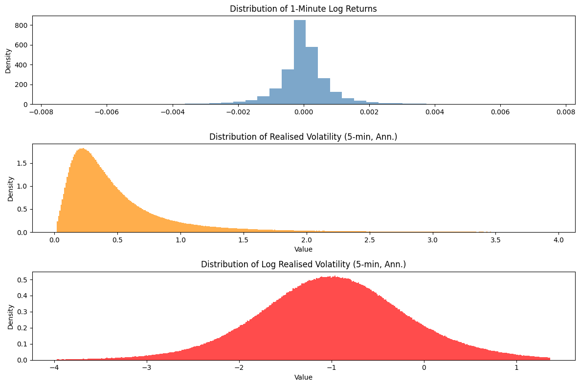
From the summary statistics, it can be seen that 1-min log returns exhibit a mean of approximately 0, as well as negligible unconditional drift and heavy tails. The 5-min RV displays a wide dynamic range corresponding to distinct volatility regimes, with extremely low value reflecting period of minimal trading activity, and an upper tail corresponding to high-volatility regimes.
With reference to figure 1, we can see that the RV is heavily right-skewed, indicating a majority of low-RV periods but episodic occurances of high-volatility spikes, which is expected of BTC market activity. With log transformation, we are able to reduce the skewness substantially to produce a more symmetrical, bell-shaped curve, which will facilitate modelling subsequently.
HAR Model Estimation Results
We specify a heterogeneous autoregressive (HAR) model to analyse how RV at multiple horizons contributes to forecasting five-minute RV at t + 5min.
\[\text{RV}_{t+5}^{(5\text{min, ann})} = \beta_0 + \beta_{5min} \text{RV}_{t}^{(5\text{min, ann})} + \beta_{60min} \text{RV}_{t}^{(60\text{min, ann})} + \beta_{1d} \text{RV}_{t}^{(1\text{day, ann})} + \epsilon_{t+5}\]The dataset was split into training and testing samples using a 80-20 split, with the model parameters estimated on the training set. From figure 1, we can see that there is a need to use Log-transformed RV instead to stabilise regression estimates by dampening the influence of extreme RV spikes on Ordinary Least Squares (OLS) estimation.
Dependent variable: $\log(\text{RV}_{t+5}^{(5\text{min, ann})})$
Number of observations: 3,528,880
Regression Coefficients, Model Fit, and Residual Diagnostics
Table 2: Regression Coefficients of HAR Model.
| Variable | Coefficient | Std. Error | t-stat | p-value |
|---|---|---|---|---|
| Intercept | -0.2196 | 0.001 | -413.8 | < 0.001 |
| log(RV_t^(5min, ann)) | 0.2169 | 0.001 | 396.9 | < 0.001 |
| log(RV_t^(60min, ann)) | 0.5738 | 0.001 | 549.6 | < 0.001 |
| log(RV_t^(1day, ann)) | 0.1974 | 0.001 | 180.5 | < 0.001 |
| Statistic | Value |
|---|---|
| Skewness | -7.386 |
| Kurtosis | 171.889 |
| Jarque-Bera | 4.23e9 |
| p-value | < 0.001 |
| Metric | Value |
|---|---|
| R^2 | 0.496 |
| Adjusted R^2 | 0.496 |
| F-statistic | 1.16e6 |
| p-value | < 0.001 |
| Durbin-Watson | 0.517 |
The model explains a substantial extent of the forecasted $\widehat{\mathrm{RV}}_{t+5}^{(5\text{min, ann})}$, as reflected in the $R^2$ value of 0.496.
From the coefficients, it can be seen that the medium-horizon $\log(\mathrm{RV}_{t}^{(60\text{min, ann})})$ dominates forecast dynamics with the largest coefficient of 0.5738. Nonetheless, the short- and long-horizon components also contribute meaningfully. All coefficients are highly statistically significant (all $p$-values $< 0.001$).
Of note, the Durbin-Watson statistic (0.517) is < 2, indicating substantial residual autocorrelation that may not be well captured by the model, and may warrant further analysis and model extensions to refine the HAR model.
Model Performance on Test Sample
Out-of-sample (n = 882,220) forecast performance is evaluated using root mean squared error (RMSE) and mean absolute error (MAE).
Test Sample Forecast Performance
Table 3: Absolute and Relative Error Metrics .
| Metric | Value |
|---|---|
| Root Mean Squared Error (RMSE) | 0.733 |
| Mean Absolute Error (MAE) | 0.420 |
| Relative RMSE | 0.791 |
| Relative MAE | 0.789 |
It can be seen from the RMSE that large forecast errors exist, resulting in RMSE > MAE. The relative RMSE and MAE show that the model outperforms a naive benchmark, proving that the HAR model provides improved performance in capturing the volatility dynamics of BTCUSDT. The error metrics are then compared to that of a naïve benchmark:
\[\widehat{\text{RV}}_{t+5}^{(5\text{min, ann})} = \text{RV}_{t}^{(5\text{min, ann})}\]Comparatively, it is notable that the relative RMSE and MAE show that the HAR model can reduce RV forecasting errors by ~20%.
Conclusion
We find that a HAR model utilising realised volatility horizons at the 5-min, 1-hour, and 1-day levels provides a statistically meaningful approach to forecasting $\widehat{\text{RV}}_{t+5}^{(5\text{min, ann})}$, with performance superior to that of a naïve persistence benchmark.
In the next stage of this study, we will address the residual autocorrelation through further model extensions to improve our forecast accuracy, before progressing to a deeper analysis of how these volatility forecasts may be translated into monetisable trading opportunities.
Citations
Wainwright, Zack. ‘A Closer Look at Bitcoin’s Volatility’. Accessed 1 February 2026. https://www.fidelitydigitalassets.com/research-and-insights/closer-look-bitcoins-volatility.
PS: GenAI was used to support the writing of this piece - but mostly for equation writing, cleaning up of markdown formatting, and language!
Comments